Replacing SQL Joins with the SAS Data Step Hash Object

So it has been a very long time since I posted on here, a lot of changes in the meantime. Long story short, I got busy, changed jobs, still busy now, but with the change in scene I have a little more motivation to blog and hopefully some more interesting things to say. I figured I’d start out by posting a quick summary of a technical presentation I gave to the SUNZ quarterly meeting late last year.

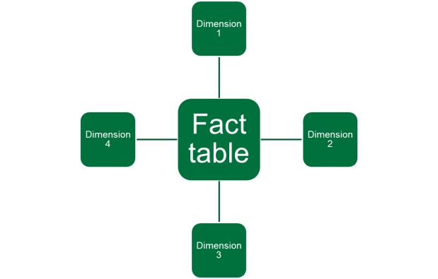
The presentation was a brief look at how to use the SAS data step hash object to replace expensive SQL joins. The scenario I had in mind was a typical one working with a data warehouse, where we join from a large, central fact table to several (typically smaller) dimension tables:

The thing is, even when the dimension tables are (relatively) small, each lookup from the fact extracts a cost, in the form of CPU time – so the more rows in the fact, the more this costs. Not only that, but as the dimensions grow (which they naturally will over time), the CPU time required for each lookup will increase. This is why the quick and easy report which took 5 minutes to run when you wrote it a year ago now keeps you (and perhaps the rest of your reporting batch) waiting for the best part of an hour.

The advantage that the hash object offers is essentially that while growth in the fact still adds to the CPU time required, growth in the dimensions does not. The hash object guarantees (except in situations involving pathological data) constant time lookup. There can be monster savings here, with some caveats which I’ll get to later. For the moment, here’s a very quick how to.

First, the (generic) SQL we’re replacing:

proc sql ;
  create table report as
  select
  	dim1.attr1
	, dim2.attr2
	, dim3.attr3
	, dim4.attr4
	, fac.measure1
  from
  	fact1 fac
	inner join dimension1 dim1
		on fac.dim1_pk = dim1.dim1_pk
	inner join dimension2 dim2
		on fac.dim2_pk = dim2.dim2_pk
	inner join dimension3 dim3
		on fac.dim3_pk = dim3.dim3_pk
	inner join dimension4 dim4
		on fac.dim4_pk = dim4.dim4_pk
		;
quit ;

The idea with using the data step hash object to replace this is simple: we add a separate hash object for each dimension, containing the keys we are using to join on and the attributes we are adding into the report table. Then for each row in the fact, if we find a match in all dimensions, we add the row into the report.

The code is as follows:

data report ;
  /* 1 - 'Fake' set statement to add variables into the PDV*/
  if 0 then set
  	fact1 (keep = measure1)
  	dimension1 (keep = dim1_pk attr1)
	dimension2 (keep = dim2_pk attr2)
	dimension3 (keep = dim3_pk attr3)
	dimension4 (keep = dim4_pk attr4)
  ;

  /* 2 - Declare hash objects for each dimension*/
  if _n_ = 1 then do ;
  	declare hash dim1 (dataset:"dimension1") ;
	dim1.definekey("dim1_pk") ;
	dim1.definedata("attr1") ;
	dim1.definedone() ;
	
  	declare hash dim2 (dataset:"dimension2") ;
	dim2.definekey("dim2_pk") ;
	dim2.definedata("attr2") ;
	dim2.definedone() ;
	
  	declare hash dim3 (dataset:"dimension3") ;
	dim3.definekey("dim3_pk") ;
	dim3.definedata("attr3") ;
	dim3.definedone() ;
	
  	declare hash dim4 (dataset:"dimension4") ;
	dim4.definekey("dim4_pk") ;
	dim4.definedata("attr4") ;
	dim4.definedone() ;
  end ;

  /* 3 - 'Join' rows to the dimensions by matching with the .find() method*/
  do until (eof) ;
  	set fact1 (keep=dim1_pk dim2_pk dim3_pk dim4_pk measure1 end=eof;
	if dim1.find() = 0 and dim2.find() = 0 and 
		dim3.find() = 0 and dim4.find() = 0 then output ;
  end ;
  stop ;

  drop dim1_pk dim2_pk dim3_pk dim4_pk ;

run ;

As per the comments, the code breaks down into 3 steps:
1 – Fake a set statement: the data step compiler does not know about the hash object when it is created, so we need to supply it with column metadata to assist with formation of the PDV.
2 – Declare and create the hash objects. The definekey, definedata and definedone methods do the work of defining the hash object, after which SAS loops over the tables named in the ‘dataset’ parameter supplied with the declare statement. For each row the key and value pairs are added into the hash object.
3 – Perform the join by matching key values from the fact table into the dimension hash objects (using the hash object find() method). This is where one fundamental difference between the two approaches becomes apparent. We’re now not joining tables on disk, as we were with the SQL join; the fact table on disk is being matched with the hash objects, which are data structures entirely resident in memory.

So is it worth it? In a word, yes – but only if you’re willing to trade off a big (sometimes huge) increase in memory consumption against the CPU time you’ll be getting back. To illustrate this, here’s some performance stats from a real-life example.

First, a small join – 2 dimensions joined to a small fact table (about 100,000 rows):

Replacing this with data step code using hash objects:

There’s a small saving in CPU time, set against a slight increase in memory consumption. It hardly seems worthwhile replacing this code, but then again it’s not a very long-running report to begin with. The real savings come when we look at the full version – this time, 9 dimensions joined to a somewhat larger fact table (~ 10 million rows). First the SQL join:

Then, the data step version:

Here, replacing the SQL code has reduced the time required by a factor of 10. This is a huge difference and we could be doing backflips and high fives all round right now, but before we kick off the celebrations, take a moment to look at the memory usage.

You’ll see that the memory consumption with the SQL code is less than 300MB, whereas the data step hash code uses a little over 10 times that. In fact, even the data step code against the small fact required over 1GB. The memory usage is linked to the size of the dimensions that you’re shoving into the hash objects, so the decrease in CPU time is being paid for more or less directly with a corresponding increase in memory. So is this a problem? Well, it might be, or it might not be. Obviously it depends on the availability of both these resources – if your server is constantly running out of memory then I’d say yes, it’s a problem. Then again, if your users are always complaining about how long it takes for their reports to run, maybe the hash object is worth a look.

I delivered a slightly longer form of this as a presentation to SUNZ last year. The slideshow is at the link below (pptx) or a pdf version is also available from the SUNZ website.

Data Step Hash Object vs SQL Join

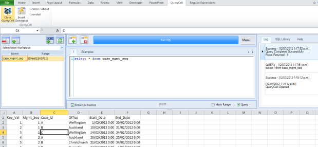
How do you SQL in Excel?

QueryCell is the Excel add-in from Oak Focus Software that brings SQL into Excel. I reviewed version 1.4 some time ago, and a few days ago lead developer Sam Howley told me about the release of version 2.0.

The new version is a complete rewrite and offers a noticeable improvement in speed, stability and responsiveness, in addition to support for 64-bit Excel. As always I’m impressed with the clean, simple look and feel of the interface, which slides out the editor when you need to use it and tucks it away when you’re done. You can manipulate data from inside the current workbook, or externally through an ODBC connection.

Sam has very kindly agreed once again to give away some free licences to Number Cruncher readers. All you have to do to get yourself one is to send me an email describing how you’ve used SQL in Excel. Could be bringing external data in through a query, or querying tables in the current workbook, could be using the Excel Data menu and MS Query to add in a connection, or scripting an ADO connection using VBA, or using QueryCell. Surprise me! Send me a description of what the information need was and how you went about resolving it.

Email me at the address at about, with ‘SQL in Excel’ in the subject line, by 10:00 pm NZDT on Saturday 14 July. I’ll judge the best/most interesting of these and publish them in a follow-up post after the weekend, so it’s important that you’re ok with other people reading what you send me.

Lags and Unintended Consequences

Analytic functions like LAG, LEAD, FIRST_VALUE and LAST_VALUE are a very useful addition to Oracle SQL, enabling retrieval of aggregate results without the need for self-joins. LAG, for instance, will allow you to get the value of a column from the previous row in a group of rows.

Here’s an example of where I used this recently. I was attempting to monitor transfers of cases between offices by reading from a table CASE_MGMT_SEQ containing a record of which offices managed which cases, which held a row for each office in the ‘management sequence’ of the case history. Here’s roughly what that looked like:

The column MGMT_SEQ tells us the position of each row in the case management sequence. Each row in the case sequence ends on the same date as the next row starts, and it is possible (although not shown in this example) for the next row to be in the same office as in the previous row. From this view we can tell that case A was managed in Wellington from Feb 1 to Feb 20 this year, then was moved to Auckland from Feb 20 to Feb 25, and finally moved back to Wellington, where it remained until Mar 10.

The SQL to track transfers needed to tell me (among other things; I’ve simplified this considerably) which case we’re transferring, when the transfer happened, where it was transferred to, and where it was transferred from:

WITH TRANSFERS AS
  (SELECT CASE_ID ,
    LAG(OFFICE) OVER (PARTITION BY CASE_ID ORDER BY CASE_ID, MGMT_SEQ) AS PREV_OFFICE,
    OFFICE ,
    START_DATE,
    END_DATE
  FROM CASE_MGMT_SEQ
  WHERE START_DATE BETWEEN TO_DATE(:STDATE, 'yyyy/mm/dd') AND TO_DATE(:ENDDATE, 'yyyy/mm/dd')
  )
SELECT 
  CASE_ID,
  PREV_OFFICE AS TRANSFER_FROM,
  OFFICE AS TRANSFER_TO,
  START_DATE AS TRANSFER_DATE
FROM TRANSFERS
WHERE (OFFICE  = :OFFICE
OR PREV_OFFICE = :OFFICE)
AND OFFICE    <> PREV_OFFICE;

The report returns for a given office any transfers in or out of a specified office over a period bounded by STDATE and ENDDATE.

But something weird is happening. I try running this report with the OFFICE parameter set to Wellington, STDATE set to 2012/02/21 and ENDDATE set to 2012/02/27, and here’s what I get:

There’s a transfer of case C from Wellington to Hamilton on Feb 24, certainly. The row where case C is managed in Wellington from Feb 23 to Feb 24 shouldn’t be counted as a transfer, as there is no previous office – the lag will return a null in this case, so the line OFFICE PREV_OFFICE in the WHERE clause will return null and hence the row will be filtered out. But there’s also case A’s transfer into Wellington from Auckland on Feb 25. There is definitely a previous office in that case. What’s going on?

The problem here is that I wasn’t paying attention to the order in which the clauses execute. It’s natural to assume that because the SELECT clause comes first, it gets executed first. In fact, the query SELECT-FROM-WHERE is executed FROM-WHERE-SELECT. This means that inside the temp table TRANSFERS, the where clause filters out rows with a start date outside the date bounds before the lag function gets to calculate the previous office. Here’s what I get when I just run the TRANSFERS sub-query with the same date parameters:

The row where case A was managed in Auckland from Feb 20 to Feb 25 is filtered out by WHERE as the start date is not within the specified bounds. Hence the window that LAG uses in SELECT to calculate the previous office has no row to look back to for the next row in the case A sequence, and this causes a null to be generated. When the WHERE clause in the outer query compares OFFICE and PREV_OFFICE, a null is returned and so this row doesn’t make it through.

So what can we do about this? Well, some people will say wrap the null values in NVL. That’s fine if you want a default value to come through, but in this case I would actually like to see the previous office – the logical fault lies in the sub-query rather than the outer query. The problem arises because the previous row is not being passed through to SELECT, so we need to get it included somehow.

In the end this was quite simple – we’re only filtering based on START_DATE, but if we include the same filter on END_DATE then the previous row will come through, by virtue of the fact that each row in the sequence ends on the same day the subsequent row starts. Here’s how the report is modified with a change to the WHERE clause in the sub-query:

WHERE START_DATE BETWEEN TO_DATE(:STDATE, 'yyyy/mm/dd') AND TO_DATE(:ENDDATE, 'yyyy/mm/dd')
  OR END_DATE BETWEEN TO_DATE(:STDATE, 'yyyy/mm/dd') AND TO_DATE(:ENDDATE, 'yyyy/mm/dd')

And the transfer from Auckland to Wellington shows up:

Reference for LAG and other analytic functions: http://psoug.org/reference/analytic_functions.html

TableCell – Beta Testers needed

Last year I posted a review of the QueryCell Excel add-in from Oak Focus Software. A few weeks ago, the developer of QueryCell let me know about a new add-in he’s developed called TableCell, a simplified version of QueryCell. Actually it was several weeks ago, sorry Sam – I’ve been a lot slower getting to this than I hoped.

Anyway, TableCell requires beta testers to do beta testing, so if you would like to help out (and get yourself some free trial software) head on over to TableCell and take a look. Basically the idea is to allow users to read from and write to database tables via ODBC. I’ve had a play and it will allow you to do just that, but not a lot more – it’s not a developer tool, it’s more aimed at the user who needs to do simple monitoring and updating without in-depth knowledge of either SQL or the data model in the DB. I see the same strength in the UI that I see in QueryCell, i.e. it’s polished, intuitive and requires minimal effort to get used to. Connecting to a DB is very easy – the one thing I would have liked to see and didn’t was a list of available tables. I know that introspection adds on a bit of overhead but in my view given the audience I see this add-in aimed at it’s probably worth it. It also requires the user to enter the name of the table’s primary key to extract data.

That’s all for now – upcoming posts over the next month include a review of some open data sources, a new Python/Excel hookup, and a brief how-to on XML data sources in Excel, which I’ll be using to build a simple currency converter.

Python Data Access patterns, part 1

Recently I’ve been reading Clifton Nock’s book Data Access Patterns: Database Interactions in Object-Oriented Applications, which as you’d expect from the title, covers a lot of patterns to do with data access. The first part of the book is dedicated to decoupling patterns, which seems to me to be pretty fundamental to good design of applications which connect with databases. If you want an application to interact with a database, then in general it’s a good idea to place the code handling data access into a separate component. The idea is to encapsulate physical database calls in logical operations, which the application can then use, as opposed to mixing them into the rest of the application code.

The benefits of keeping application code (code which needs to know about objects in the application domain) separate from data access code (code which needs to know about how to get at the database) are many. Maintenance is a lot easier – by exposing only logical operations to your application you can change anything related to the detail of how these are implemented without worrying about breaking code elsewhere in the application. The application code itself is cleaner, as it can focus on the objects without worrying about how these are stored physically. This also affords a nice division of labour, so you could have someone working on the business logic in the application who knows nothing of the database behind it.

Here’s an example of how such a data access component could be implemented in Python, where the application is interacting with a SQLite database. The DataAccessor class (apologies to Clifton Nock here, I both stole the class name and modelled the code pretty closely on his Java version) handles connecting to the database and exposes the operations the application might require: read, insert, update, delete. For the sake of brevity I’ve only included the read and insert operations here – update and delete follow a pretty similar pattern to insert.

import apsw
import os

def sql_trace(stmt, bindings):
    'Echoes all SQL executed'
    print "SQL:", stmt
    if bindings:
        print "Bindings:", bindings
    return True

class DataAccessor(object):
    '''
    Class to handle data access using apsw sqlite wrapper
    '''
    def __init__(self, dbpath, echo=False):
        try:
            if os.path.exists(dbpath):
                self.conn = apsw.Connection(dbpath)
                self.cur = self.conn.cursor()
                if echo:
                    self.cur.setexectrace(sql_trace)
            else:
                raise IOError('Database not found: ' + dbpath)
        except apsw.CantOpenError as detail:
            print "Unable to open db file: ", dbpath, detail
            raise

    def read(self, table, columns=None, where_row=None, sort_cols=None):
        '''Executes a SELECT statement against table.

        Arguments:
        table                 -- name of the table to be read
        columns (optional)    -- list of columns to be read
                              from table
        where_row (optional)  -- dict used to build WHERE
                              clause
        sort_cols (optional)  -- list of (column, order) pairs
                              used to specify order of the
                              rows returned. Needs to be of
                              the form ('<column>', 'ASC'|'DESC')

        Returns: rows returned from the SELECT statement.
        '''
        try:
            stmt = 'SELECT '
            if columns:
                stmt += ', '.join(columns)
            else:
                stmt += '*'

            # from clause
            stmt += "\nFROM " + table

            # where clause
            if where_row:
                stmt += "\nWHERE "
                stmt += "\n  AND ".join([col + "=:" + col \
                                    for col in where_row])

            # order clause
            if sort_cols:
                stmt += "\nORDER BY "
                stmt += ', '.join([col[0] + ' ' + col[1] \
                                    for col in sort_cols])

            stmt += ';'

            # submit and return results
            args = where_row and (stmt, where_row) or (stmt,)

            results = columns and [dict(zip(columns, row)) \
                for row in self.cur.execute(*args)] \
                or [row for row in self.cur.execute(*args)]

            return results

        except apsw.SQLError as sql:
            print 'Error in SQL submitted:', sql
            print 'SQL:', stmt
            if where_row:
                print 'Bindings:', where_row

        except apsw.Error as error:
            print 'APSW Error: ', error

        except Exception as error:
            print 'Error reading from database:', error

        finally:
            self.cur.close()

    def insert(self, table, values):
        '''Executes an INSERT statement against table.

        Arguments:
        table           -- name of the table to be written to
        values          -- list of rows (dicts) to be inserted

        Returns: None
        '''
        try:
            # build list of column names
            cols = values[0].keys()

            # generate insert statement
            stmt = 'INSERT INTO ' + table + ' ('
            stmt += ', '.join(cols)
            stmt += ') VALUES ('
            stmt += ', '.join([":%s" % col for col in cols])
            stmt += ')'

            # submit

            self.cur.execute('BEGIN IMMEDIATE')
            self.cur.executemany(stmt, values)
            self.cur.execute('COMMIT')

            return self.conn.changes()

        except apsw.SQLError as sql:
            print 'Error in SQL submitted:', sql
            print 'SQL:', stmt
            self.cur.execute('ROLLBACK')

        except apsw.Error as error:
            print 'APSW Error: ', error
            self.cur.execute('ROLLBACK')

        except Exception as error:
            print 'Error submitting insert:', error
            self.cur.execute('ROLLBACK')

        finally:
            self.cur.close()

I’ve used the apsw SQLite wrapper here, but if at some point I decided to switch to pysqlite, or to use a MySQL database, I could do so without greatly affecting the calling code. The potential drawback here is that what you gain is offset by the loss of control. It may well be that all your application needs to do is to read from or write to a single table at a time, but what about if it needs to execute a join? Drop or create a table or view? What if you need to do specify a more complex where condition than “column=value”?

It may well be possible to rewrite this class to expose these operations, but I could see this getting to be a lot of work. In the next part I’ll look at some ORM (Object Relational Map) solutions which get around this nicely by mapping an OO structure to a relational model.