Building an Excel currency converter, part 3

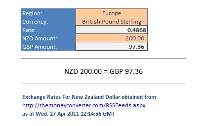
OK, now to finish off the converter! In the previous post in this series, we’d managed to extract the rate and the description from the rates table, which we’d imported in the first part from an xml source. Now we get to put that rate to use. The end goal (which is the bit that the user will be interacting with) looks something like this:

This is made up of 3 input cells (Region, Currency and NZD_Amount) and 3 output cells (Rate, Converted_Amount and Display). I’ll handle the input cells first.

All have data validation (Data -> Data Tools -> Data Validation) specified. For NZD_Amount this is simple. Validation criteria are Allow:= Decimal, Data:= greater than, Minimum:= 0. I’ve also added in an input message, with Title:= “NZD Amount”, and Input message:= “Enter amount to be converted.”

Region and Currency have slightly more complicated criteria. Both are drop-down lists of values, populated from the rates table. The complications arise partly because Currency is dependent on Region – that is, the values available in the Currency drop-down depend on the value that’s been selected in the Region drop-down. Some additional complications: the currencies available in Rates_Table change from time to time. There are some which are always included, but others are not. Also, the currencies are sorted within the table by title, rather than region, which makes getting a list of currencies for a particular region tricky.

We’ll start with the easy bit, getting a list of regions. I simply copied the ‘category’ column from the rates table, pasted it onto the Reference sheet, and with the pasted values selected, used the ‘Remove Duplicates’ tool (Data -> Data Tools -> Remove Duplicates) to get a list of 7 distinct regions. I name this range as ‘category’ and then use it as a source for validation of the Region input cell:

Now to get the Currency values to go with the selected Region. Ideally we’d have the same sort of input for the data validation dialog – a contiguous range of cells to select from. In order to do this, I decided to sort Rates_Table – by category, then by title. This means that Rates_Table now displays the currencies in blocks according to the regions. The trouble is, when the query is refreshed, this sort order will be replaced by the order supplied by the xml source. So I added a code module ‘MSortRatesTable’ to the project, and entered the very simple SortRatesTable macro into it:

Sub SortRatesTable()
'
' SortRatesTable - Sorts Rates Table
'

    With ThisWorkbook.Worksheets("Rates").ListObjects("Rates_Table").Sort
        .Header = xlYes
        .MatchCase = False
        .Orientation = xlTopToBottom
        .SortMethod = xlPinYin
        .Apply
    End With

End Sub

In the ThisWorkbook class module, I then hook the AfterXmlImport event to ensure that every time the xml source for the table is refreshed, the table is sorted:

Private Sub Workbook_AfterXmlImport(ByVal Map As XmlMap, _
                                    ByVal IsRefresh As Boolean, _
                                    ByVal Result As XlXmlImportResult)
If IsRefresh Then
    SortRatesTable
    Application.Calculate
End If
End Sub

Now, to use this newly sorted table. Directly to the right of the named range ‘category’ (recall this was where the regions were stored on the Reference sheet) I enter this formula:
=ADDRESS(MATCH(category,Rates_Table[category],0) + 12,6,,,"Rates") &":"& ADDRESS(MATCH(category,Rates_Table[category],0) + 12 + COUNTIF(Rates_Table[category],category) - 1, 6)

Let’s break this down:
MATCH(category,Rates_Table[category],0) + 12 uses implicit intersection with the category range to return the first row where the category value occurs in the category column in Rates_Table, with 12 added on to account for the additional 12 rows above the table, including the header.

ADDRESS(MATCH(category,Rates_Table[category],0) + 12, 6,,, “Rates”) takes this row value, 6 for the column where the currency column is included in Rates_Table (F), and the name of the sheet where Rates_Table to return the address of the first cell in the currency column corresponding to the region specified by category – e.g. ‘Rates!$F$13’ is the address of the first African currency in the table.

ADDRESS(MATCH(category,Rates_Table[category],0) + 12 + COUNTIF(Rates_Table[category],category) – 1, 6) does much the same, but adds the number of rows in the table corresponding to the category, minus one, to return the address of the last cell in the range of currencies belonging to the region specified by category.

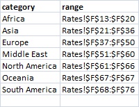
Putting this together with a colon in between the two addresses, we get the address of the entire range of currencies for each region. Here’s what this looks like on the Reference sheet:

This entire range I name ‘range_lookup’. Then, in validation for the Currency input cell, as with Region, I set Allow:= List, but for Source I use the formula:
=INDIRECT(VLOOKUP(Region, range_lookup, 2, FALSE))
VLOOKUP returns the address corresponding to the selected region from range_lookup, which INDIRECT then converts into a range for Excel to use as the Source array.

So that takes care of the input cells, which leaves the 3 output cells, Rate, Converted_Amount and Display. These are fairly uncomplicated – Rate has the formula:
=VALUE(INDEX(Rates_Table[rate], MATCH(Currency, Rates_Table[currency], 0)))

MATCH gives the row number matching Currency in the currency column of Rates_Table, which INDEX then uses to find the relevant rate in the rate column. VALUE then converts this (which RXGET had provided as a character string) to a numeric value.

Converted_Amount uses the formula =NZD_Amount*Rate, which is fairly self-explanatory. However in the label for the cell I’ve used a little trickery to display the 3-letter code for the selected currency (e.g. GBP for British Pounds), like so:
=LEFT(INDEX(Rates_Table[title], MATCH(Currency, Rates_Table[currency], 0)), 3)&" Amount:"

The 3-letter code is the first 3 letters of the title column in Rates_Table. I use the same formula to help format the Display output:

=TEXT(NZD_Amount, "[$NZD] #,##0.00") & " = " & TEXT(Converted_Amount, "[$" & LEFT(INDEX(Rates_Table[title], MATCH(Currency, Rates_Table[currency], 0)), 3) & "] #,##0.00")

And that’s that. For anyone who’s curious to see the finished product, I’ll edit this and upload it shortly.

Building an Excel currency converter, part 2

To recap where we left off in the first part, we’d managed to import xml data from the rss feed for NZD rates at themoneyconverter.com into a table (which I’ve named Rates_Table). This gave us a list of rates which we can use – however the format is not quite right. In the “description” member of “item”, the rate is expressed in a structured text format, like so: “1 New Zealand Dollar = 2.96886 Argentine Peso”. Now of course that would be useful as it is, if I were prepared to manually type out the 2.96886 part myself to convert from NZ dollars to pesos. Which of course I’m not, lazy data analyst that I am.

What I’m going to do instead is to extract the two relevant parts of that text, the two bits that I need to know: the rate (the numeric bit, in this case 2.96886) and the foreign currency description (the character string that comes after the numeric bit, in this case “Argentine Peso”). This is something that can be done with text functions like MID and FIND in Excel, of course, and this is a perfectly legitimate way to go about it. However, unless you can find a really clever way to do it, you’ll end up with a really long, convoluted and awkward formula. Which is a great reason to use regular expression functions instead. RXGET for instance, is designed to do exactly this sort of extraction. Here’s how I went about it:

First, we need to determine the regular expression pattern that fits the text. The pattern I chose is
=\s(\d*\.\d+)\s(.+)
or to break it down a little,

1. an equals sign followed by a space: =\s;
2. followed by a group, which in turn contains zero or more digits, followed by a decimal point, followed by one or more digits: (\d*\.\d+) This will be used to capture the rate part of the expression. Note that the decimal point needs to be escaped here, as it signifies an arbitrary character in a regular expression;
3. followed by another space: \s;
4. followed by a second group, which contains one or more arbitrary characters: (.+) This will capture everything after the space, which in this case will be the currency description. Here the decimal point should not be escaped as we need it to match any character.

Once I know that this pattern works, I add a new sheet titled ‘Reference’ and enter the pattern into a cell that I name Rate_Pattern. Now I can use it to extract the rate and the currency using RXGET. I add a column with the header rate at the right-hand end of the Rates_Table and enter in it the RXGET formula, with the following arguments:

This corresponds to the formula:
=RXGET(Rate_Pattern,Rates_Table[[#This Row],[description]],1).
Note that the Submatch argument has the value 1, as we’re extracting the 1st matched group from the expression. To get the currency description, in another new column with the header currency I enter the same formula with the Submatch argument changed to 2 to extract the second group. So here’s how the table looks right now (click on the image to take a closer look):

In the final part of this series I’ll complete the converter by adding in a selector to pick out a rate from the table by specifying the currency.